Cuts and graphs, again

Remember that a is the separation of edges that partitions the vertices into two non-empty groups. These vertices need not be connected.

s-t graphs

Say that we had a directed graph, with a special source $s$ with only outgoing edges and a special sink $t$ with only incoming edges. This is what we define as an s-t graph. The weights on the edges are capacities. We will talk more about these later.

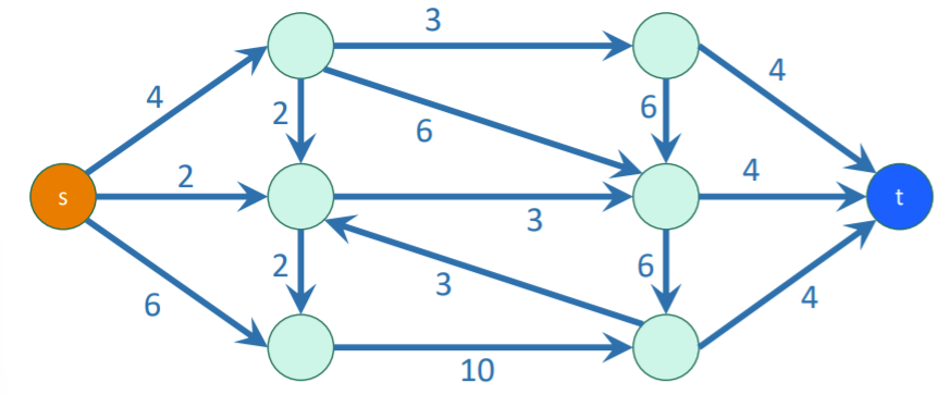
s-t cuts

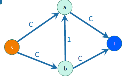
an s-t cut is a cut that separates $s$ from $t$. We call an edge as crossing the cut if it goes from $s$ to $t$. Note that this doesn’t include edges that go the other way. The capacity of a cut is the sum of capacities that cross the cut (again, not including things that go the other way)

Key question: can we find a cut that has minimum capacity? Historically, this has uses in the military. Given a graph of railroad connections, how many do we have to interrupt before we seal off a city? (if we interpret a greater capacity as harder to interrupt)

Flows

We can understand the capacity of each edge as the limit of transportation (like the railroad example), we can define a flow of an edge as how much of this capacity is already taken over. There are two key rules of flows

1. The flow on an edge must be less than or equal to its capacity

2. The flow going into a vertex must be the same as the flow going out of a vertex. This is the formalism:

The maximum flow is a flow that shuttles as much “things” from $s$ to $t$ as possible.

Max flow min cut

Here is a key weird observation that we will spend some time proving: the maximum flow is also the minimum capacity that you need to cut. We call this the max-flow min-cut theorem

Intuitively, this makes sense. In the maximum flow situation, you are limited by the bottleneck on some graph. When you want to minimize the capacity in a cut, you would be going for the bottleneck.

Lemma 1: max flow $\leq$ min cut

If we make any s-t cut, then we separate out a group of vertices including $s$, from another group of vertices including $t$. Any sort of flow must go from this group $S$ to the group $T$ (capital letters denote the groups). The highest flow would be the saturation of these edges. This is the value of the cost of the cut.

So, the key upshot is that the flow across any s-t cut is at most the cost of the cut. Therefore, we conclude that at the min-cut, the maximum flow (which is just another flow) just be at most the cost of the min-cut.

• A rigorous proof

  This proof feels a little “hacky” but it does show the importance of “nonoperations” in proofs. We start from the simple definiti noof flow, which is

  

  The second sum is zero because we don’t flow into a source, but we keep it here for the next step. Our next step realizes that the net flow into and out of any node in $S$ (the large set) is zero, so we can add an external summation

  

  This is non-zero, because a neighbor $x, y$ might be OUTSIDE of $S$ and flow into the group.

  Next, we realize that we can separate the neighbors into two groups: ones from $S$ and ones from $T$.

  

  Now, because nodes flowing within $S$ will sum to zero, we only care about the nodes

How do we show equality?

Well, we can do this through the Ford Fulkerson algorithm!

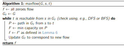
Ford-Fulkerson algorithm

Our intuition is this: just take the largest possible flow at each step from $s$ to $t$. While this might work in some cases, the greedy approach can sometimes fail to converge at the right solution, because sometimes you need to walk back on certain flow to get a net gain in flow.

Residual graph

The FF algorithm relies on the concept of a residual graph. In the image below, the left is the normal graph (with the flows marked) and the right is the residual graph.

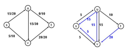
This residual graph $G_f$ has the same vertices as the original, but there is a forward + backward edge for every directed edge. The backward edges represent how much flow you need to take away to get zero flow in the original graph. The forward edges represent how much flow you need to add to maximize the flow in the original graph edge.

The key insight

if there exists a path from $s$ to $t$ in the residual graph, then we can further augment the total flow in the original graph

This is easy to understand if every edge on the path in $G_f$ is a forward edge, because that increase the flow on all the edges, including the edge that begins on $s$ and the edge that ends on $t$,.

But this is still the case if there are some backward edges. Because a path from $s$ to $t$ necessairly has an outgoing edge from $s$ and an incoming edge on $t$. So we are increasing the net flow, because that’s how we are measuring it. Running through a backward edge means walking back on a past choice for the greater good.

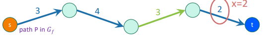
The algorithm

Basically, you want to find a path in $G_f$ and increase/decrease the flow by the smallest limit in the path. We call this the augmenting path

Termination and cuts (proving max-flow min-cut)

Here, we try to prove the max-flow min-cut theorem.

We can terminate the algorithm once $s$ and $t$ are no longer in the same connected component.

Let’s cut the graph into two vertices: things reachable from $s$ in $G_f$ and things not reachable from $s$, which includes $t$.

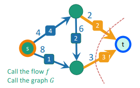
All of the flow must cross this cut if we are to get to $t$. But more importantly, the edges in this cut are full. Why? Because the forward edges are non-existent in $G_f$, else these components wouldn’t be disconnected!

From these two points, we must conclude that the cost of the cut is the same as the maximum flow, as desired.

Dealing with multiple sources and sinks

Just make a “master” source and a “master” sink that connects to all the sources and sinks, respectively. The weights between the master and source/sinks should be $\infty$

Complexity of Ford Fulkerson

If you picked arbitrary paths you can actually get into a very long loop and you end up augmenting by one step at a time. No matter what, FF algorithm will terminate correctly, but some choices are slower than others.

• Example

  

  Here, if you keep on crossing the middle a-b edge to augment the path, you will end up with $c-1$ augmenting steps

Here’s another interesting observation: if all the capacities are integers, then all the max flows are integers. This is because we only add and subtract integers

Therefore, in the most naive case, we have the complexity as $O(m|f|)$, where $|f|$ is the maximum flow. This is because the BFS takes $O(m)$ time, and we augment the flow by at least one each time.

Now, the problem comes on how we can design an algorithm that doesn’t depend on $|f|$ in its runtime

Edmonds-Karp

We can use BFS to find the nodes reachable from $s$. The idea is that you always pick the shortest path. You have $O(m)$ for a BFS, and thanks to a nice lemma, the total number of times an edge can disapear from $G_f$ is at most $n/2$. Therefore, the total runtime is $O(m^2n)$, where the $m$ comes from the BFS, the other $m$ comes from the total edges, and $n$ comes from the previous lemma.

Application: maximum matching

Simple assignment

Say that we had a bipartite graph with students on one side and preferred outfits on the other. If we can only give one outfit to each student, how can you maximize happiness? D

Here, the easiest solution is to solve it through maximum flow, using a universal source and sink. All edges have capacity 1

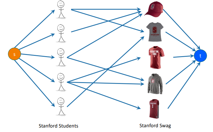
The capacity of 1 from the $s$ make sure that each student can only take one clothing. The capacity of 1 to the $t$ make sure that each clothing can be assignied to only one student

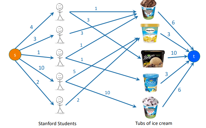
Constrained assignment

There people and ice cream flavors. Each ice cream $i$ has $k_i$ scoops. Each person $j$ can consume at most $m_j$ scoops. Each person selects a set of ice cream they want, and they also upper-bound the ice cream flavors. For example, a person can want 10 scoops but they can only tolerate 2 scoops of Chocolate.

We can represent this as a max-flow problem too! The edges from $s$ represent consumption limits, and the edges to $t$ represent the ice cream capacity. Each edge from person to ice cream has a capacity, which is the maximum they want to consume. An edge exists from person to ice cream if this person has a non-zero tolerance for it.

What problems can be solved through maximum flow?

Typically, these problems deal with “more is good” but there is a capacity on the “more”. In other words, there must be a constraint that prevents people from being totally happy, and we are trying to optimize based on this constraint.

More examples

• the hard part is getting the assignment from friend to friend

• Connect $s→v_i$ if friend $i$ paid below average. The weight is the amount of money they owe

• Connect $v_j→t$ if friend $j$ paid above average. The weight is the amount of money they need to get back

• Connect each $v_i$ (money-owing person) to $v_j$ (money-lacking person) (it’s a bipartite graph) with edge weight infinity (or any number larger than the maximum transaction between them)