Greedy Algorithms

Let’s compare and contrast this with divide & conquer and dynamic programming. Greedy algorithms make a singular choice and then never look back. In contrast, backtracking and DP often reduce a large problem into a series of smaller problems and then condense them.

It’s best to understand it through a graph, actually

What doesn’t work

Greedy algorithms don’t work when doing the best now doesn’t necessairly correspond to what is good later. A classic example is the unbounded knapsack problem.

A greedy approach would be to take items that are of the highest cost to weight ratio and fill up the bag that way. If you fill the bag all the way to the top, then this works perfectly fine. However, if there is any room left over, you could be in trouble. Say that you had gold bars of weight 10 and value 100, and silver bars of weight 7 and value 60, in a knapsack of limit 25.

• Greedy approach will put two gold bars and stop at weight 20 and value 200

• Correct approach would put one gold bar and two silver bars and stop at weight 24 and value 100 + 2 * 60 = 220.

The general framework

How can we tell that a greedy algorithm works or not? Well, we can do it inductively.

We want to show that, for every subproblem decomposition, there is still some way of creating an optimal solution from the given path so far. Or, to think about it another way: given an optimal solution $T^*$ and a greedy choice, we can always modify $T^*$ to agree with the greedy choice without changing optimality.

So here is some general tips

1. base case should be obvious: if we make no choices, the optimal path remains

2. if the greedy algorithm agrees with $T^*$, then you are good

3. If the greedy algorithm disagrees with $T^*$, then you need to show that you can essentially manipulate $T^*$ such that it agrees with the greedy choice while maintaining optimality

Tips and tricks

Often the proof draws from the two narratives

• By making the greedy choice, you are doing something minimally or maximally

• By making the optimal choice, you are doing something else that may be maximal and minimal

• you want to show that from your greedy choice, you can mess with the optimal choice to constrain it to the greedy selection without changing optimality

Example 1: optimal scheduling

Suppose that you are given a list of bounds $[s, f]$ that represent the starting and finishing times of different activities in a schedule. If you wanted to do the most activities without any intersection, can we design an algorithm for this?

The DP approach

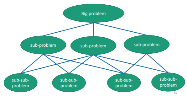
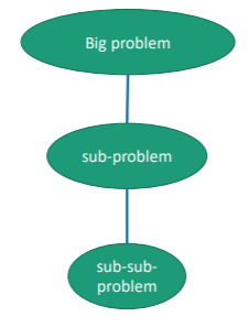
If we define $A_{ij}$ as the maximum subset of non-conflicting activities that start after activity $a_i$ and finish before activity $a_j$, we can derive the following DP approach

But this makes an $n^2$ table, which means that the total complexity is $O(n^3)$. Can we do better?

The greedy insight

If we are building problems from left to right, as soon as you put down a $f$, you can’t put down another activity that has $f' < f$ . So, you want to grow $f$ as slowly as possible. To do this, just the activities by the finishing time. Then, moving from smallest to largest $f$, put down activities that don’t intersect.

The proof of correctness

Base case: with no selection, there is obviously an optimal path.

Given an optimal selection so far, and given a $T^*$ that completes the optimal selection (given from some oracle):

1. If the next selected activity agrees with the next activity in $T^*$, we are all set

2. If the next selected activity disagrees, we need to think about it for a second. Let’s say that greedy picks $a_k$ and optimal picks $a_j$. We know that $f_k < f_j$, so $a_k$ doesn’t intersect with the next element in the sequence of $T^*$, the one after $a_j$. Therefore, we can just swap out $a_j$ for $a_k$ in $T^*$ without any conflict.

Because the next greedy selection doesn’t contradict optimality, we are done with the induction.

Example 2: Scheduling

Say that you had a bunch of things to do that take $t_i$ hours, and for every where that passes until task $i$ is done, you pay $c_i$. You want to arrange your schedule to minimize the total costs.

The greedy insight

You can show algebraically that if job $A$ takes $x$ hours and costs $z$ per hour, and job $B$ costs $y$ hours and costs $w$ per hour, we are comparing the following equations

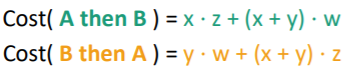
If you expand this out, you will see that the larger of the ratio of $\frac{w}{y}$ as compared to $\frac{z}{x}$ determines which one is better. Intuitively, this is cost of delay / time it takes. The more it costs to delay, the better it is to do first. Similarly, the less time it takes, the better it is to do first.

From this insight, we can look at pairwise values if the schedule. If each pair is ordered by their ratios, then we can just order the entire schedule by the ratios.

tl;dr sort the schedule items by increasing $delay cost/ time$. This takes $O(n\log n)$ time.

Proof of correctness

We can look at pairwise swaps (see below) because swapping two jobs doesn’t impact the times of the jobs around it!

Base case is obvious.

Inductive case, let’s say that we have a disagreement. Say that the greedy algorithm chooses $B$ while the previous optimal chooses $C$. Let’s say that currently, the order of the optimal is $C→A→B$.

We know that $B$ has the highest ratio (by the greedy algorithm). Therefore, the ratio of $B$ is at least as much as $A$. However, we know that $A$ can’t be lower in ratio than $B$, because if that’s the case, we can swap $B$ and $A$ and yield a better cost tuple of $A, B$.

Let’s pause for a second. We established the upper bound of $A$ from how the greedy algorithm picked the job. We established the higher bound of $A$ from the optimality condition of the optimal solution. Therefore, we must conclude that the ratio of job $A$ must be the ratio of job $B$. As such, we can switch the two jobs in the optimal ordering without sacrificing optimality.

We continue this argument until $B$ moves back to where $C$ was

Example 3: Huffman Coding

The key observation: some letters are used more than other languages in the english language, and so they contain less information. Can we represent this with our coding formulation?

We want to encode the most common characters in as little characters as possible. However, we must also keep things unambiguous. In other words, we can’t represent $A$ as $0$ and $B$ as $00$. This is because we are no longer encoding strings with a set number of bits.

Encoding tree and expected cost

The best encoding strategy is to use a tree whose edges represent a binary choice and whose leaves represent each letter. To decode, you traverse the tree based on the binary digit you encounter, and then when you reach a leaf, you write down that character. Conversely, you can search the tree and create encodings for each letter (think depth-first traversal).

We define the expected cost as the expected length of a character. We compute this through

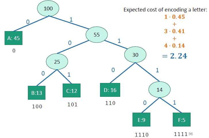
Greedy insight

Take the least frequent letters (or groups of letters) and combine them to form another node. This is because we want to greedily build the subtrees from the bottom up, with the less frequent letters forming the deeper trees (think about the expectation: we relegate the deeper things to the lower probabilities).

Proof of correctness

We want to show that in each step, we are not ruling out an optimal answer. Let’s start with the first step.

We claim that if $x, y$ are the two least-frequent letters, then there is an optimal tree where $x, y$ are siblings.

So let’s use a similar swapping argument. Suppose that an optimal tree looked like this

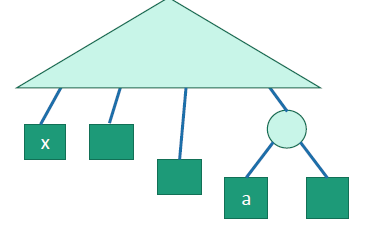
We know that $a$ is more frequent than $x, y$ by definition. Therefore, if we switch $a$ and $x$, the cost can’t increase because we are moving a more common letter to a more shallow point in the tree.

And this is true for all $a \neq x, y$, so we can keep swapping until $x, y$ are next to each other.

Now, we continue by showing that optimality is preserved with groups. We can treat the groups as leaves in the new alphabet, with frequencies that are the aggregate of the letters of its children. Then, we can use the lemma from before.

The big idea is that we show that the least two elements can be grouped together while keeping optimality. And you can keep on paring the tree down until you reach the root, which yields the optimal solution.

Additional problems

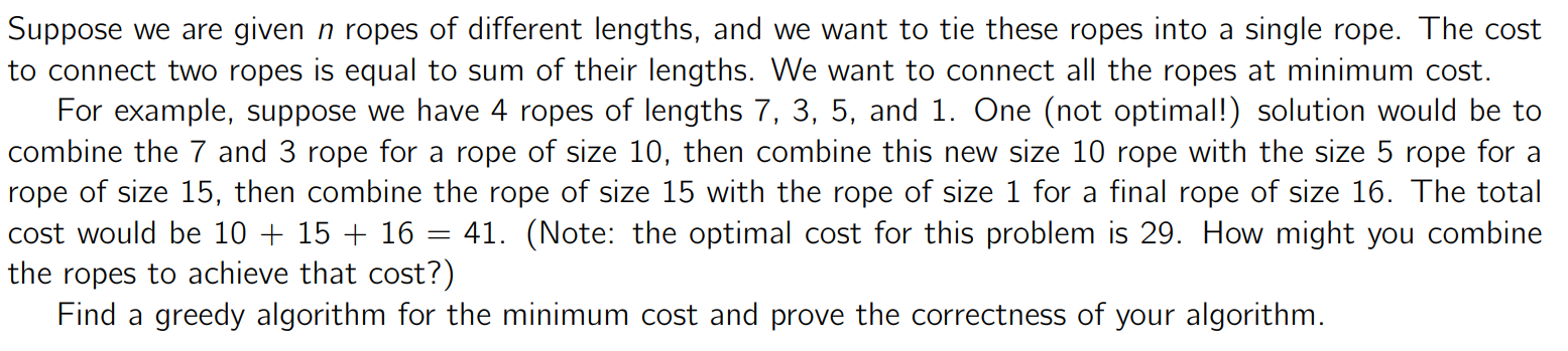
The greedy algorithm is to just pick the shortest ropes to combine. This yields essentially the huffman encoding problem again. We want to show that if we select the two smallest ropes, there exists an optimal path.

The greedy algorithm selects $x, y$ tie together, while the optimal algorithm selects $a, b$ to tie together. Because $x, y \leq a , b$, we know that swapping the ropes out for $a, b$ can’t increase the final cost. It can’t decrease the cost either, else the optimal solution isn’t actually optimal. Therefore, there exists an optimal path, and inductively, this means that the greedy algorithm yields an optimal path.

The greedy algorithm is to keep a list of colors used so far (initially empty) and iterate through the nodes one by one. We color the node a color that hasn’t been used by the neighbors yet. If all colors on the list have been used, we add another color. It doesn’t always use the least number of colors, though

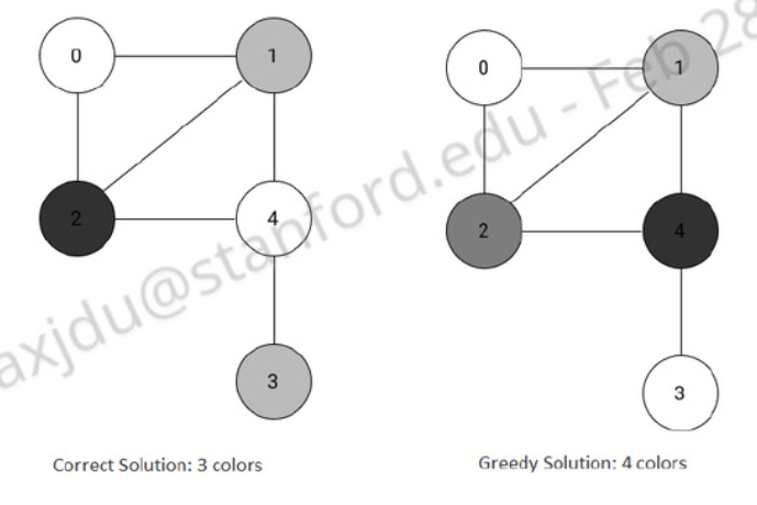
We do know that this never uses more than $d + 1$ colors. Every time we select a vertex to color, it has some $k$ neighboring vertices. In the worst case, each of the vertices have a different color. Therefore, coloring in this vertex would require a $k + 1$st color. Therefore, the colors needed to color some node is $\leq k+ 1$. We know that $k \leq d$, so the total number of colors needed is $\leq d + 1$.