The big idea

We can use decision trees to show upper bounds on sorting algorithms.

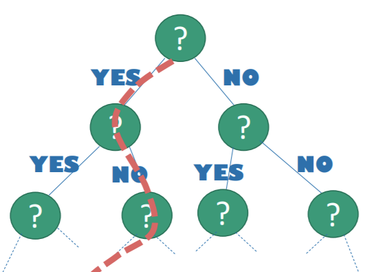
Decision tree

In comparison based sorting, we are allowed to compare two elements at a time and understand if one is larger or smaller than the other. You can think of this as a decision tree in which each node is a question, and each answer gets you to another question until you reach the end.

Minimal complexity

Now here’s the crux: at the end, the algorithm spits out a sorted array. If the array of size $n$, then there must be $n!$ sorted array at the leaves of the tree. If we started with one question (which we do) and if the tree is binary & balanced, then the longest path must be $\log_2(n!)$

From Stirling’s approximation or the neat trick with log factorials, we get hat $\log(n!) = \Theta(n\log n)$.

So if the general comparison based sorting algorithm is lower bounded with $n\log n$ in the worst case, then we can assert that all such algorithms must run in at least $n\log n$. Cool!

Randomized algorithms

You can actually prove that the expected runtime of randomized algorithms like Quicksort also have the same lower bound. However, we will not do it here (a little beyond the scope of our discussion)

Understanding the tree

One Philosophy

Perhaps this is the most unintuitive part of the whole thing. How do you even begin thinking of a problem in terms of a decision tree? Well, it always helps to think of the number of possible inputs and the number of possible outputs.

Here’s the general rule of thumb: the number of leaf nodes is the input size divided by the number of inputs that can reach one output.

It’s best to think of a leaf node as containing the “answer” to something. Let’s look at a few examples

1. Sorting a list: the leaf node contains a list of indices that map an input to sorted output

2. Select top-K in a list: the leaf node contains a list of indices that are the top-k in the list

3. Merging sorted list: the leaf node contains a list of insertion orders

4. $\sqrt{n}$-sorting (in which the sorted number may be within a certain radius of the actual location): the leaf node contains a list of indices that map to an approximately sorted output

Now, let’s think about the number of inputs that can reach one output. Practically speaking, this is the number of inputs for which, after you apply the leaf node’s list of indices, yield a correct answer.

1. Sorting a list: there can only be one ordering of numbers that work with the root node’s sorting plan. So, there are $n!$ leaf nodes

2. Select top-K in a list, sorted. If you specify the indexes of top-k, the other $n-k$ numbers can be permuted any way you want. So there are $n! / (n-k)! = \binom{n}{k}k!$ leaf nodes

3. Select top-K in a list, unsorted. If you specify the indexes of top-K, firstly, there are $k!$ different permutations of top-k elements that yield the correct answer. Second, there are $(n-k)$ different permutations of non-top-k elements that don’t matter. So, you have $n!/(n-k)!k! = \binom{n}{k}$ leaf nodes

4. Merging sorted lists of size $n, m$. Here, you must work backwards. If you give an order of insertion, only one pair of lists will satisfy (assuming distinct numbers). But how large is the input? Well, you can imagine splitting apart a sorted sequence of size $m+n$. You can do this in $\binom{m+n}{n} = \binom{m+n}{m}$ different ways.

5. $\sqrt{n}$ sorting: there are $n!$ inputs, but you can show that there are $O(n^n)$ different valid sort outputs. You can imagine turning this relationship around and saying that there are $O(n^n)$ different inputs that reach one output. Therefore, the number of leaf nodes is $\frac{n!}{O(n^n)}$

From the number of leaf nodes, we just take the logarithm to find the depth of the tree

At the end, you will get an expression that should be placed in $\Omega$, as it is the lower bound.

Another philosophy

Just look at the number of outputs an algorithm can make

1. In sorting, it’s just $n!$

2. In select top-K, sorted, it’s just $\binom{n}{k}k!$, because you pick the top k, and then you sort

3. In select top-K unsorted, it’s just $\binom{n}{k}$

4. In merging sorted lists, the algorithm picks which ones to merge at what time, so it’s just $\binom{m+n}{n}$

5. In $\sqrt{n}$ sorting, there are $O(n^n)$ possible correct outputs, so you can imagine the best algorithm as taking advantage of the multiple paths and pushing $O(n^n)$ different inputs down one solution path. Therefore, there are $n!/O(n^n)$ leaf nodes.